Are electric cars a worse investment ?

This post examines the value depreciation of electric vehicle (EV) in the Montreal area, with an analysis of the impact of the Quebec government’s decision to phase out the Roulez Vert program on the value.

Electric vehicles (EVs) are generaly more expensive than their gasoline counterpart. Yet, adoption has still be relatively high thanks to governement incentives and the cheap cost of electricity in the province of Quebec. But, as the Roulez Vert program from the government of Quebec is slowly getting phased out, it is worth examining more precicely the financial impact of EVs. The program’s initial goal was to promote EVs with monetary incentives (up to $7,000 CAD for new cars and $3,500 CAD for used cars). Removing this program means that every EV purchased starting on January 1, 2025, will be more expensive.

This presents a unique opportunity for acquiring an EV this year with a lower value depreciation than what would traditionally be expected, as the cost of EVs will slowly increase over the next few years. That is, of course, under the assumption that the cost of new EVs will remain relatively stable over the next few years.

My understanding of EVs is that they should hold value longer than your typical gasoline vehicle. There are fewer parts involved in the engine, and the battery capacity can remain relatively stable over a huge number of recharge cycles. The brake pads can be changed less often thanks to the regenerative braking system. Rusting should be roughly similar to gasoline vehicles. The main disadvantage is that battery capacity has been increasing significantly with every new generation of EVs. Therefore, there is an incentive to upgrade your car and thus saturate the used EV market, which decreases prices and depreciates the value of the car faster.

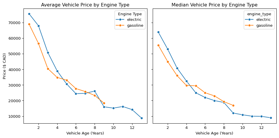
Before making any assumptions, it is best to refer to data to see how, with a constant government incentive over the past few years, the EVs in the Montreal market area have been depreciating in value using gasoline vehicles as a baseline.

Acquiring used vehicle market data

To do so, I first scraped some used vehicle market data using the Web Scraper Chrome extension. I then used the US car models GitHub repository to parse the vehicle make and model out of the text description for each vehicle.

Here are the first 5 rows of this new dataset:

# Code for parsing us-car-models-data (make and models)
us_car_models_df = None
for file in glob.glob("data/us-car-models/*.csv"):
    current_year = pd.read_csv(file)
    if us_car_models_df is None:
        us_car_models_df = current_year
    else:
        us_car_models_df = pd.concat([us_car_models_df, current_year])

all_cars_models = us_car_models_df.model.unique().tolist()
all_cars_models = sorted(all_cars_models, key=len, reverse=True)

# Code for parsing scaped vehicle data
evs = pd.read_csv("data/electric_cars.csv")
gas = pd.read_csv("data/gasoline_cars.csv")
evs["engine_type"] = "electric"
gas["engine_type"] = "gasoline"
df = pd.concat([evs, gas]).drop_duplicates()

df["vehicle-name"] = df["vehicle-name"].str.strip()
df["year"] = df["vehicle-name"].str[:4].astype(float)
df["price"] = (
    df["price"].str.extract("([\d,]+)", expand=False).str.replace(",", "").astype(float)
)


df = df[df["year"] > 2010]
df["make"] = df["vehicle-name"].str.extract("\d+\s+([A-Za-z\-]+)\s", expand=False)

def find_model_in_paragraph(text):
    reg = re.compile('[^a-z0-9]')
    for model in all_cars_models:
        if reg.sub('', model.lower()) in reg.sub('', text.lower()):
            return model
    return None

df["model"] = df["vehicle-name"].apply(find_model_in_paragraph)

df["mileage"] = df.mileage.str.replace("[km,]", "", regex=True).astype(float)
df["vehicle_age"] = 2025 - df.year
df.drop(
    ["vehicle-name", "vehicle-desc", "pagination", "web-scraper-order", "web-scraper-start-url"], axis=1, inplace=True
) # drop unwanted columns
df.dropna(inplace=True)
df.year = df.year.astype(int)

print(df.head(5))
df["MakeModel"] = (df["make"] + " " + df["model"]).astype("category")

<>:23: SyntaxWarning: invalid escape sequence '\d'
<>:28: SyntaxWarning: invalid escape sequence '\d'
<>:23: SyntaxWarning: invalid escape sequence '\d'
<>:28: SyntaxWarning: invalid escape sequence '\d'
/tmp/ipykernel_2584/632754913.py:23: SyntaxWarning: invalid escape sequence '\d'
  df["price"].str.extract("([\d,]+)", expand=False).str.replace(",", "").astype(float)
/tmp/ipykernel_2584/632754913.py:28: SyntaxWarning: invalid escape sequence '\d'
  df["make"] = df["vehicle-name"].str.extract("\d+\s+([A-Za-z\-]+)\s", expand=False)

   mileage    price engine_type  year       make      model  vehicle_age
0  27707.0  24995.0    electric  2022      Mazda      MX-30          3.0
1   5923.0  58995.0    electric  2023       Audi  Q4 e-tron          2.0
2  66068.0  22988.0    electric  2018  Chevrolet    Bolt EV          7.0
3  45669.0  30985.0    electric  2020        Kia     Optima          5.0
4  39169.0  38895.0    electric  2022    Hyundai        Ion          3.0

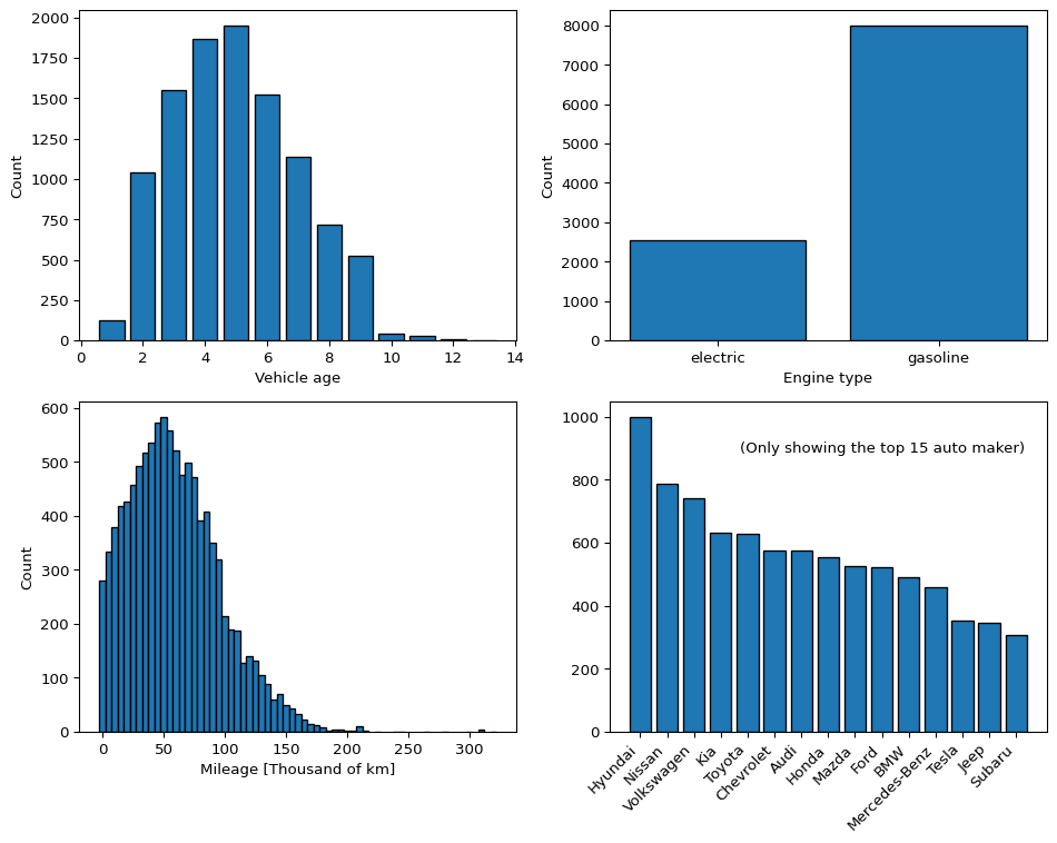
Data visualization

We can start our analysis with some visualization of this newly created dataset.

fig, axs = plt.subplots(2, 2, figsize=(10, 8), tight_layout=True)

# Vehicle age
hist_data = np.unique(df.vehicle_age, return_counts=True)
axs[0][0].bar(*hist_data, edgecolor="black", align="center")
axs[0][0].set_xlabel("Vehicle age")
axs[0][0].set_ylabel("Count")

# Engine type
hist_data = np.unique(df.engine_type, return_counts=True)
axs[0][1].bar(*hist_data, edgecolor="black", align="center")
axs[0][1].set_xlabel("Engine type")
axs[0][1].set_ylabel("Count")

# Mileage
bin_size = 5000
bins, counts = np.unique(df.mileage.astype(int)//bin_size, return_counts=True)
bins *= bin_size
axs[1][0].bar(bins/1000, counts, edgecolor="black", align="center", width=bin_size/1000)
axs[1][0].set_xlabel("Mileage [Thousand of km]")
axs[1][0].set_ylabel("Count")

# Top 15 auto maker
bins, counts = np.unique(df.make, return_counts=True)
top_idx = np.argsort(counts)[::-1]
bins = bins[top_idx[:15]]
counts = counts[top_idx[:15]]
axs[1][1].bar(bins, counts, edgecolor="black", align="center")
axs[1][1].set_xticklabels(bins, rotation=45, ha='right')
axs[1][1].text(9, 900, "(Only showing the top 15 auto maker)", va="center", ha="center")
pass

Histogram for each column of the dataset.

To examine the effect of engine type on vehicle price depreciation, we can calculate both the average and median prices for vehicles of varying ages.

fig, axs = plt.subplots(1, 2, figsize=(10, 5), tight_layout=True, sharey=True)

avg_price_by_age = df.groupby(['vehicle_age', 'engine_type']).price.mean().reset_index()
med_price_by_age = df.groupby(['vehicle_age', 'engine_type']).price.median().reset_index()

# Plotting
sns.lineplot(data=avg_price_by_age, x='vehicle_age', y='price', hue='engine_type', marker="o", ax=axs[0])
sns.lineplot(data=med_price_by_age, x='vehicle_age', y='price', hue='engine_type', marker="o", ax=axs[1])
axs[0].set_title('Average Vehicle Price by Engine Type')
axs[1].set_title('Median Vehicle Price by Engine Type')
axs[0].set_xlabel('Vehicle Age (Years)')
axs[1].set_xlabel('Vehicle Age (Years)')
axs[0].set_ylabel('Price ($ CAD)')
axs[0].legend(title='Engine Type')
pass

Modeling

To validate this conclusion, I created a simple linear mixed-effect regression model to predict vehicle prices using mileage, age, and engine type. There are some biases that are unaccounted for: the options added to the vehicle and the MSRP. We still can get a rough estimate by inspecting the parameters of the learned model of the impact the engine type has on value depreciation.

import statsmodels.formula.api as smf

model = smf.mixedlm("price ~ engine_type*mileage + engine_type*vehicle_age", df, groups="MakeModel").fit()

print(model.summary())

                             Mixed Linear Model Regression Results
================================================================================================
Model:                         MixedLM             Dependent Variable:             price        
No. Observations:              10521               Method:                         REML         
No. Groups:                    619                 Scale:                          89864076.3370
Min. group size:               1                   Log-Likelihood:                 -113024.6370 
Max. group size:               239                 Converged:                      Yes          
Mean group size:               17.0                                                             
------------------------------------------------------------------------------------------------
                                        Coef.       Std.Err.    z    P>|z|   [0.025     0.975]  
------------------------------------------------------------------------------------------------
Intercept                                81613.909  2876.868  28.369 0.000  75975.351  87252.467
engine_type[T.gasoline]                 -15252.574   902.110 -16.908 0.000 -17020.677 -13484.471
mileage                                     -0.099     0.007 -13.400 0.000     -0.113     -0.084
engine_type[T.gasoline]:mileage              0.024     0.008   2.806 0.005      0.007      0.040
vehicle_age                              -3347.532   158.521 -21.117 0.000  -3658.227  -3036.837
engine_type[T.gasoline]:vehicle_age        639.121   177.666   3.597 0.000    290.902    987.341
MakeModel Var                       4744113322.490 29685.324                                    
================================================================================================

What’s most interesting about the results are the coefficients. We notice that, as expected and on average, every km driven (mileage) decreases the value of the vehicle by $0.097 and every year added decreases it by $3,333.58. The model uses EVs as a baseline, and we can notice that gasoline vehicles increase the value of the car by $0.022 for every km and $628.86 for every year. Now, these numbers are inexact; the relationship between these variables is most likely not linear. The sign of the coefficient is, however, undeniable: gasoline vehicles hold their value longer than their electrical counterparts.

Conclusion

It is evident that EVs undergo greater depreciation than gasoline cars. However, this difference appears primarily in vehicles older than 5 years. Five years ago marked a significant increase in the popularity of EVs in Canada, notably with the release of the Tesla Model 3. The technology has advanced considerably since then, and it is somewhat expected that the early models of EVs did not perform well in the market and are thus resold at lower values.